
Following on from Coronavirus, which is a matter of some immediacy, I'm going to try to provide a more basic approach to the study of this sort of modelling.
Daniel Bernoulli, way back in 1760, did some thinking on this, based on data collected most of a century earlier by John Graunt [1].
A general population has birth and death going on anyway but, looking for a simple model to start with, one could contemplate a disease that works relatively quickly, like measles or ebola, such that only the infection is relevant.
Seeking very simple models we might postulate a fixed population, so that we declare the birth and death rates to be equal or zero. Consider a population, initial size X₀, whose size, X, is expressed by the function x(t). Then a disease causes a loss, and we have a model very similar to
dx/dt = - kx where k is the infection rate.
Slightly more advanced, imagine k is replaced by a function. For some infection µ(t) that removes people from the population in some sense, we can write the rate of change in X as:
dx/dt = - µ(t).x(t) a product of functions in t.
By separation of variables we get something very like the expression for integrating factors in the pages on differential equations, that x = X₀ exp( - integral µ(t) dt = X₀ exp(H(t)) where we could call H(t) some sort of accumulated hazard. [1, P3]. This gives an idea of a general form of the expected modelling equation.
In general the birth rate and the death rate are different and are affected differently by circumstances. Where a disease is modelled whose speed (cause of death) is similar to those of 'normal' deaths, one is looking at additional deaths; mostly we choose to ignore this. Because different factors affect the two parts (birth and death), so where they are considered at all they are often indicated separately. I have written several pages on related topics; essays 208 and 240, but also essays 173 - 175.
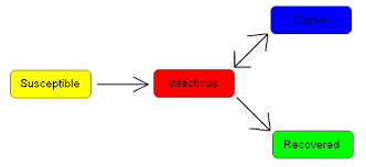
Quite clearly during the progress of a disease the total population is made up of three groups, where I have given the usual labels—that is, I called them something different at first but then found a text that agreed with what I'd scribbled.
S, those at risk of catching the disease, to be thought of as Susceptible
I, those currently infected, who are able to pass the disease to the susceptible group. I have used the character 𝙸 below to help it be distinguishable.
R, those who are removed from the infection, either by recovering or by immunisation or by dying. These are the people who cannot pass the disease on.
Obviously the total population N, is N= S+I+R where each of S,I & R are functions in time. Equally obviously, to those who have read the pages on D.E.s, the differential of N is zero, so S' + 𝙸' + R' = 0, so we might hope to produce a system of equations representing this. For swiftly acting epidemics, this is a suitable assumption.
The idea of counting those cured or dead together, so becoming Removed (or whose cases have in some way become Resolved, producing a Result) leads us to the idea of the reproduction number, usually denoted R₀, which represents the number of people each infectious person will infect. R₀>1 causes the disease to spread; R₀=1 represents an endemic disease, since each infected person infects one other, so the population infected stays constant; R₀<1 means the disease dies out.
We will need two variables of the sort we can measure and use to describe an epidemic:
(i) something to represent how fast people become infected. We use 𝞫 to represent the number of people each infected person infects per time period. We assume that all people are equally likely to contract the disease, however untrue that might be; what I think of as 'intense' models will contemplate the population as made up of many overlapping but different sub-populations, so that we can then model, for example, the effect of the epidemic within a hospital (a sub-population) and perhaps look at how many useful staff might be sacrificed to treating the outbreak. More particularly, one would model how disastrous it is to lose any of the front-line specialists. So in any time unit each infected person is able to transmit the disease to 𝞫N others; if you prefer to look at that another way, the fraction of the population infected in the next time period is 𝞫. The only others who may contact the disease is the fraction S/N. The fraction of the population removed from the susceptible group are those infected, so I think dS/dt is the product of 𝞫N, S/N and 𝙸/N, and that therefore dS/dt = - 𝞫 S 𝙸 / N which seems dimensionally consistent with a rate of people per time unit. I found a different version of this that looked wrong, but could be explained by assuming that the population sums to unity, so that S and 𝙸 continue to be fractions of the population. That does simplify the initial algebra.
(ii) something representing the death or recovery rate, which we could perhaps also view as the time to a result. To be consistent with 𝞫 we want a rate, (or something we can consider as a fraction of the population) so the convention is to use 𝞬 to indicate the rate at which we gain a result (either death or recovery). Since 𝞬 is a rate measured in people per time unit, then the reciprocal, 1/𝞬, is expressed in time units per person and represents the mean infectious period. This suggests a fairly simple model where R₀ is simply 𝞫 /𝞬.
Within the SIR model for the time being, we can see that dR/dt = 𝞬 𝙸
Since N=S+I+R was a fixed population, dN/dt=0 = dS'dt + d𝙸/dt + dR/dt and in the absence of an alternative, d𝙸 /dt = 𝞫S𝙸/N - 𝞬𝙸
As [2] points out, the notion of a fixed population succeeds here if infection is very much quicker than the rates of birth and death (which you might construe mathematically as competing infections). So other versions of the SIR model treat the cases where births and deaths are considered, those where there is no immunity, or where immunity can occur in births or where immunity is not permanent or, perhaps the most worrisome, where there is a period in which the infected person is both asymptomatic and infectious.
Another, simpler, model simply says that the susceptible group is simply everyone who is not currently infected. That would apply to infections like colds, for which recovery does not imply immunity. Such a model gives d𝙸/dt = 𝞫 𝙸 (1- 𝙸) which is a standard A-level problem where ln ( 𝙸 / (1- 𝙸) = c + 𝞫 t. You supply initial conditions and express 𝙸(t).
A slight improvement gives d𝙸/dt = 𝞫 𝙸 (1- 𝙸) - µ 𝙸 where the µ 𝙸 term represents some people already being immune or becoming immune by virtue of recovery. This leads to the population being as infected as it can be without reaching unity, that is, the first differential has a later zero value. In this model R₀ is, I think, 𝞫/µ.
I hope to return to this topic armed with better tools.
The infectious period can create difficulties, because it demands that there be some sort of time delay inserted as an additional factor in each of S', 𝙸' and R'. Enter source [3], which explains this a little. ¹ Using F' to indicate dF/dt, the author has used the simpler representations S' = -𝞫SI; R' = 𝞬 𝙸 and therefore 𝙸' = 𝞫S𝙸 - 𝞬𝙸. He, Ignasi Gros, describes 𝞫 and 𝞬 as the contagion and recovery parameters respectively. If we want to model that the newly infected folk are not yet infectious for time 𝜏, and, that in this period they cannot recover. So the decay element will be of the form e⁻ᵏᵗ, (but kt will be 𝞫𝜏) representing that the infectious people were infected 𝜏 earlier, — and we need to offset t to t-𝜏 too. This is not a multiplier, but a changed value to be applied, S (t-𝜏) rather than S(t).
Thus the adjustment is to S' (and, in consequence, 𝙸') such that S' = -𝞫SI becomes S' = -𝞫 S(t) I(t-𝜏) e-𝞫𝜏 where that last element is also written exp(-𝞫𝜏) just in case your system has dropped the superscript. Similarly we can insert the same factor (t-𝜏) exp(-𝞫𝜏) into R' because recovery is also delayed, which makes 𝙸' have this as a common factor, so that 𝙸' = (exp(-𝞫𝜏) ) 𝙸(t-𝜏) ( (𝞫 S(t) -𝞫) [3, slide 44].
Alternatively we can look at incubation period quite differently, by dividing our whole population into not three groups but four: the Susceptible, the Exposed, the Infected and the Resolved. The exposed are infected but not infectious and they are not in a position to recover. So in the same way that 1/𝞬 represented the mean infectious period, so now 1/𝞽 represents the incubation 'rate'. So the system of equations is S' = -𝞫SI; R' = 𝞬 𝙸; and the two new equations are E' = 𝞫SI - 1/𝞽 E and 𝙸' = 1/𝞽 E - 𝞬𝙸. You can see that these still add to zero. Initial conditions, for those bothered by this (I'm in the habit of considering such far later) would make S₀ > 0, E₀ and I₀ ≥ 0 and R₀ = 0. Gros continues to look at those who are Asymptomatic
DJS2020127
top pic found hurriedly via Google, but I'd prefer the red box to be labelled Result, Resolved or Removed.
I found very much more success than with these mathematical models by messing about with a spreadsheet. If you'd like a version of that, do ask. As regards Covid-19, I have been putting updated charts here through the period of the infection in the UK, and while the presentation of the graphs varies by the week in response to the data, this (Excel) modelling is more satisfactory, in the sense that I can easily display what is and show versions of what will be. Clearly we'd like for R₀ to move below 1, but the spreadsheet model shows that the disease dies out because it runs out of new people to infect, even when R₀>1. I found predictions that looked acceptable (yet no deaths are 'acceptable') for several values of 1<R₀<2. This brings us to a far better understanding of the expression 'herd immunity', so easily misunderstood, as evidenced by our remarkably non-numerate press. Glaring exception, ITV's Robert Peston (Balliol, PPE; ITV 2016-now; I ought to buy his books).
2 https://en.wikipedia.org/wiki/Mathematical_modelling_of_infectious_disease
3 https://www.slideshare.net/IgnasiGros/delaydifferential-equations-tools-for-epidemics-modelling
¹ I was hugely frustrated that much of what I wanted to read was hidden behind pricing barriers which do not exist for those employed in academia. So much for 'information wants to be free'. I would see this as an exciting module within a university course, lending itself to extensive modelling, not least those extensively using computing power. DJS 20200127
I found [3], with which I disagreed with quite a lot of the maths as shown, especially slide 21. Slide 37 is dimensionally rubbish unless the declared 𝞪 and 𝞫 have different units. However, slides 40-45 and 46-55 do show how to model incubation periods, delayed infectiousness and the asymptomatics (possible carriers).
Q1 𝞪 = 𝞫 suggests to me that both are zero. This is inconsistent with Bernoulli saying a = b = ⅛.
Q2 𝙸(t) = ( 𝙸₀ exp( 𝞫 t) ) / ( 1 - 𝙸₀ + 𝙸₀ exp(𝞫 t) ) very clumsy to type without use of script editors.
Essay 293 - Covid-19 charts charts published daily reflecting concerns and issues.
Essay 291 - Effects of an outbreak what it says, effects, but some description of what we have (and not)
Coronavirus (Y10+) modelling problems
Epidemics more general theory
Infectious disease looking at the 2020 problem, particularly effects of the reproduction number changing.
Viruses are very small